Week 7 – Lightcurves in the time of Coronavirus

Now that society has collapsed, I finally have had some time to read some papers. We’ll get to that later in this post, but first I’ll review some small changes to my pipeline, our group’s intended schedule for pipeline convergence, an additional lightcurve I made, and some notes on two resources our adviser asked us to summarize.

The first update I made was to our crossmed function, which actively prints the shifts between two images as they are computed. Previously, the function would also print the “max” shift for a given list of images, but this maximum was quite literally a maximum, so if an image had large negative shifts in either coordinate, these weren’t expressed in the print statement. Lena had some concerns about her shifts as we were moving to align our images to the same image (in our case, we chose to align to the first R-band image taken in each field, because the signal to noise of these images was larger than the signal to noise of the H-alpha images), so in order to compare our shifts I wanted accurate print statements on this function. I changed that quickly by using the “numpy.absolute” function.

Lena and I plan to convene after class Wednesday to discuss how we intend on stitching our pipelines together. Before then I want to fix the alignment issues that were causing the large error bars in the previous post’s light curves.

Our adviser was kind enough to give us a spreadsheet of the AAVSO certified variable stars in our two fields, Taurus and TESS Sector 21, Camera 1. We took a peak at Taurus last week, so this past week I’ve investigated the singular known variable star in the TESS field: FN Cnc.

Commonly, the names for well known variable stars are formatted following the General Catalogue of Variable Stars (GCVS) first published by Boris Kukarkin et al. in 1969 in the Soviet Union. This nomenclature prefaces the star’s name with “V*” and objects are identified within a constellation by two letters, pertaining loosely to its position, counting up from AA to ZZ. This way I can tell just from it’s name that V* FN Cnc is a known variable star somewhere nested in the constellation of Cancer.

Variable stars will be classified if their lightcurves, colors, or other behaviors resemble that of another well studied variable. T Tauri stars, which are an important category of Pre-Main-Sequence stars (think: baby suns), are named after the star T Tauri. Looking up FN Cnc’s profile in the American Association of Variable Star Observers’ (AAVSO) database, the international Variable Star Index (VSX), I found that FN Cnc is an RR Lyrae variable with a period of 0.5135751 days.

The titular RR Lyrae was discovered by Williamina Fleming at the Harvard Observatory at the turn of the century, and “RR Lyrae” variables are noted for their short periods (hence FN Cnc’s half a day period), large amplitude oscillations (according to the VSX, FN Cnc ranges from 15.4 – 16.71 magnitudes in V Band), and asymmetric variation (as we’ll see). These stars are evolved off the main sequence and onto the Horizontal Branch. This implies they are burning helium at their cores; helium burning in the star’s core causes the star’s opacity to increase with increased temperature via the kappa mechanism. This oscillatory process causes the temperature of the variable star to fluctuate: as helium atoms are partially ionized the star becomes more opaque, trapping photons in the star, which then put a net pressure on the star, forcing it to expand. Once the star has expanded sufficiently, it can release this pressure and slowly cool as it contracts, before it contracts enough that it’s temperature then re-ionizes its helium, increasing it’s opacity, and the cycle continues.

Like last week I threw our observing run TESS images into AIJ (this time using the R-band images) and plopped an aperture over FN Cnc before commanding the computer return me the relative flux of the aperture as compared to 30 other randomly selected stars in the field. Instead of spending time with AIJ’s lightcurve figure plotter I exported the table of results to a text file, which I then brought up in python.

I knew the period of FN Cnc from it’s VSX entry, so I wanted to make a standard, phase shifted lightcurve. This process takes the period of the variation as known and plots all the data point as if they occurred within the same period. If I did this correctly I could expect to see a single sharp peak with the slow decrease in flux as typical of RR Lyrae stars. To phase shift the data points I created a quick python function, which I ran on Julian Dates for each image using a period of 0.5135751 and a t0 equal to timestamp of the maximum data point.

#define phase shift function
def phaser(data, t0, period):
    phases = [] #empty list for results
    for d in data: #iterate for each data point given
        phi = ((d - t0)/period)%1 #compute phase modulo 1, in order to get 
                                  #phases between 0 and 1
        phases.append(phi) #append computed phase to list
    return phases

I then plotted two of these phases (in order to better illustrate the periodic nature of the variation), producing a standardized light curve.

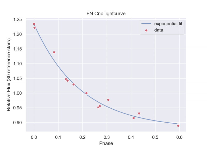
While it appears we hadn’t the luck to catch any of the upswing of the variation, we’ve certainly been successful in observing an RR Lyrae light curve! On a whim, with no scientific justification, I decided to try and fit a curve to this data, because it looked to me like it could be easily fit by an exponential decay. Doing so yielded the next plot,

which looks pretty neat. Maybe some day I’ll learn a bit more about RR Lyrae variables and their functional form, but until then I’ve slaked my desire to put curves atop data points.

I entered this video having an ok grasp on the fourier transform, and in some ways I felt like I left it more confused than when I entered. In my mind, I understood that any given function or signal can be constructed as a sum of sine and cosine functions, and the fourier transform was the mathematical operation that decomposes a function into those sine and cosine functions. The fourier transform takes a function or data as input and returns a function of frequency, the magnitude of which expresses the importance of any frequency sine wave in constructing the input.

3B1B’s “winding machine” provides an explanation for all the moving parts within the fourier transform, but it didn’t feel like it had a physical impetus. I wasn’t quite sure how the winding machine carried any meaning outside of a collection of different intuitions about the fourier transforms. In that way, it didn’t really unify the various intuitions the video was adept at illustrating, and so I was left wondering how these different pieces were physically motivated or connected. I did find his explanation of the “persistence” of a frequency modifying the magnitude of the fourier transform helpful, because that was something that I hadn’t considered before.

This reading was hefty and quite thorough, so here I’ve included by “best of” notes, or the things that I found most helpful.

Frequency & period resolution: df = 1/(N*D), dP = P^2/(N*D), where N is total number of samples and D is the space between samples. This explains why both more finely sampled data and larger data sets increase the resolution of a given lightcurve.

Fast Fourier Transform (FFT): a method for computing the fourier transform quickly that works for evenly sampled data only! I didn’t know this was a stipulation – I’m curious how this might affect our implementation of the fourier transforms with our data.

Fourier analysis is useful for analyzing stars with multiple periods. An example of this is the RR Lyrae variables we discussed previously, which have a known second order variation called the Blazhko effect.

Autocorrelation compares points separated by various intervals in order to reveal the strengths of different period fits.

In order to keep up with recent science, I was tasked with finding 2-3 recent papers that seemed relevant to my project. My discoveries are linked below with a short description of the paper.

The most applicable prize goes to “Accretion in low-mass members of the Orion Nebula Cluster with young transition disks” by de Albuquerque et al. 2020, which was pushed to arXiv today (Tuesday, March 24th). This paper seeks to measure accretion in low mass Young Stellar Objects (YSOs) in the Orion Nebula cluster using VLT/X-shooter data. From their sample of five, they measure accretion in three very low mass Orion members, two of which they could confirm hosted circumstellar disks. This paper was accepted for publication.

Another applicable paper was “Accretion Properties of PDS 70b with MUSE” by Hashimoto et al. 2020, which was pushed to arXiv a week ago (March 17th). It presents an accretion rate that does not agree with previous estimates; their estimate puts the accretion rate of PDS 70b an order of magnitude higher than it’s host PDS 70, which (to me) is disturbing, frightening, and very interesting. They used a ratio of H-alpha to H-beta flux to determine their accretion rate. This paper has also been accepted for publication.

Until next week, clear skies!